December 15, 2012

政党と政策の距離の可視化

政党間の類似度の可視化で使ったデータを標準化して特異値分解して可視化．双対尺度法とか数量化理論III類とかコレスポンデンス分析とか言われている．たしか．

図 ◆政策，■政党．政策とそれに賛成する政党が近くにある…はず

以下コード

政党間の類似度の可視化

日本政治.comの投票マッチングから各政党の政策に関する質問に対する姿勢から，政党間の距離を計算し可視化してみた．

各質問に対して賛成・中立・反対を 1, 0, -1 で表し各政党をベクトル化
ベクトル間のユークリッド距離を計算
多次元尺度構成法で可視化（Pythonで多次元尺度構成法を実装してみる，Excelの散布図のデータにラベルをつける）

ただし以下に注意

各質問の重みは考慮していない
距離の定義を変えればまったく異なる見え方に

さらに政党と政策との距離も可視化してみた→政党と政策の距離の可視化

以下コード

やっつけなのでてきとう
あとで双対尺度法試してみる
一つ前に書いた要約プログラムで連立政権について考えてみる

December 14, 2012

インストール

Homebrewでインストール

brew install mongodb
==> Downloading http://fastdl.mongodb.org/osx/mongodb-osx-x86_64-2.2.2.tgz
######################################################################## 100.0%
==> Caveats
To have launchd start mongodb at login:
    ln -sfv /usr/local/opt/mongodb/*.plist ~/Library/LaunchAgents
Then to load mongodb now:
    launchctl load ~/Library/LaunchAgents/homebrew.mxcl.mongodb.plist
Or, if you don't want/need launchctl, you can just run:
    mongod
/usr/local/Cellar/mongodb/2.2.2-x86_64: 20 files, 170M, built in 98 seconds

上にあるようにログイン時に起動してロードするには

ln -sfv /usr/local/opt/mongodb/*.plist ~/Library/LaunchAgents
launchctl load ~/Library/LaunchAgents/homebrew.mxcl.mongodb.plist

起動

mongod

接続

mongo

チュートリアル

> use mydb
switched to db mydb
> db
mydb
> j = {name: 'mongo'};
{ "name" : "mongo" }
> k = {x: 3}
{ "x" : 3 }
> db.things.insert(j)
> db.things.insert(k)
> show collections
system.indexes
things
> db.things.find()
{ "_id" : ObjectId("50caeb1fdab5ce4e84a41f78"), "name" : "mongo" }
{ "_id" : ObjectId("50caeb29dab5ce4e84a41f79"), "x" : 3 }

ループで挿入

> for (var i = 1; i <= 20; i++) db.things.insert({x:4, j:i})
> db.things.find()
{ "_id" : ObjectId("50caeb1fdab5ce4e84a41f78"), "name" : "mongo" }
{ "_id" : ObjectId("50caeb29dab5ce4e84a41f79"), "x" : 3 }
{ "_id" : ObjectId("50caeee0dab5ce4e84a41f7a"), "x" : 4, "j" : 1 }
{ "_id" : ObjectId("50caeee0dab5ce4e84a41f7b"), "x" : 4, "j" : 2 }
{ "_id" : ObjectId("50caeee0dab5ce4e84a41f7c"), "x" : 4, "j" : 3 }
{ "_id" : ObjectId("50caeee0dab5ce4e84a41f7d"), "x" : 4, "j" : 4 }
{ "_id" : ObjectId("50caeee0dab5ce4e84a41f7e"), "x" : 4, "j" : 5 }
{ "_id" : ObjectId("50caeee0dab5ce4e84a41f7f"), "x" : 4, "j" : 6 }
{ "_id" : ObjectId("50caeee0dab5ce4e84a41f80"), "x" : 4, "j" : 7 }
{ "_id" : ObjectId("50caeee0dab5ce4e84a41f81"), "x" : 4, "j" : 8 }
{ "_id" : ObjectId("50caeee0dab5ce4e84a41f82"), "x" : 4, "j" : 9 }
{ "_id" : ObjectId("50caeee0dab5ce4e84a41f83"), "x" : 4, "j" : 10 }
{ "_id" : ObjectId("50caeee0dab5ce4e84a41f84"), "x" : 4, "j" : 11 }
{ "_id" : ObjectId("50caeee0dab5ce4e84a41f85"), "x" : 4, "j" : 12 }
{ "_id" : ObjectId("50caeee0dab5ce4e84a41f86"), "x" : 4, "j" : 13 }
{ "_id" : ObjectId("50caeee0dab5ce4e84a41f87"), "x" : 4, "j" : 14 }
{ "_id" : ObjectId("50caeee0dab5ce4e84a41f88"), "x" : 4, "j" : 15 }
{ "_id" : ObjectId("50caeee0dab5ce4e84a41f89"), "x" : 4, "j" : 16 }
{ "_id" : ObjectId("50caeee0dab5ce4e84a41f8a"), "x" : 4, "j" : 17 }
{ "_id" : ObjectId("50caeee0dab5ce4e84a41f8b"), "x" : 4, "j" : 18 }
Type "it" for more
> it
{ "_id" : ObjectId("50caeee0dab5ce4e84a41f8c"), "x" : 4, "j" : 19 }
{ "_id" : ObjectId("50caeee0dab5ce4e84a41f8d"), "x" : 4, "j" : 20 }

カーソル操作

> var c = db.things.find()
> while (c.hasNext()) printjson(c.next())
{ "_id" : ObjectId("50caeb1fdab5ce4e84a41f78"), "name" : "mongo" }
{ "_id" : ObjectId("50caeb29dab5ce4e84a41f79"), "x" : 3 }
{ "_id" : ObjectId("50caeee0dab5ce4e84a41f7a"), "x" : 4, "j" : 1 }
{ "_id" : ObjectId("50caeee0dab5ce4e84a41f7b"), "x" : 4, "j" : 2 }
{ "_id" : ObjectId("50caeee0dab5ce4e84a41f7c"), "x" : 4, "j" : 3 }
{ "_id" : ObjectId("50caeee0dab5ce4e84a41f7d"), "x" : 4, "j" : 4 }
{ "_id" : ObjectId("50caeee0dab5ce4e84a41f7e"), "x" : 4, "j" : 5 }
{ "_id" : ObjectId("50caeee0dab5ce4e84a41f7f"), "x" : 4, "j" : 6 }
{ "_id" : ObjectId("50caeee0dab5ce4e84a41f80"), "x" : 4, "j" : 7 }
{ "_id" : ObjectId("50caeee0dab5ce4e84a41f81"), "x" : 4, "j" : 8 }
{ "_id" : ObjectId("50caeee0dab5ce4e84a41f82"), "x" : 4, "j" : 9 }
{ "_id" : ObjectId("50caeee0dab5ce4e84a41f83"), "x" : 4, "j" : 10 }
{ "_id" : ObjectId("50caeee0dab5ce4e84a41f84"), "x" : 4, "j" : 11 }
{ "_id" : ObjectId("50caeee0dab5ce4e84a41f85"), "x" : 4, "j" : 12 }
{ "_id" : ObjectId("50caeee0dab5ce4e84a41f86"), "x" : 4, "j" : 13 }
{ "_id" : ObjectId("50caeee0dab5ce4e84a41f87"), "x" : 4, "j" : 14 }
{ "_id" : ObjectId("50caeee0dab5ce4e84a41f88"), "x" : 4, "j" : 15 }
{ "_id" : ObjectId("50caeee0dab5ce4e84a41f89"), "x" : 4, "j" : 16 }
{ "_id" : ObjectId("50caeee0dab5ce4e84a41f8a"), "x" : 4, "j" : 17 }
{ "_id" : ObjectId("50caeee0dab5ce4e84a41f8b"), "x" : 4, "j" : 18 }
{ "_id" : ObjectId("50caeee0dab5ce4e84a41f8c"), "x" : 4, "j" : 19 }
{ "_id" : ObjectId("50caeee0dab5ce4e84a41f8d"), "x" : 4, "j" : 20 }

カーソルで配列の操作

> var c = db.things.find()
> printjson(c[4])
{ "_id" : ObjectId("50caeee0dab5ce4e84a41f7c"), "x" : 4, "j" : 3 }
> c.toArray()
[
 {
  "_id" : ObjectId("50caeb1fdab5ce4e84a41f78"),
  "name" : "mongo"
 },
 {
  "_id" : ObjectId("50caeb29dab5ce4e84a41f79"),
  "x" : 3
 },
 {
  "_id" : ObjectId("50caeee0dab5ce4e84a41f7a"),
  "x" : 4,
  "j" : 1
 },
 {
  "_id" : ObjectId("50caeee0dab5ce4e84a41f7b"),
  "x" : 4,
  "j" : 2
 },
 {
  "_id" : ObjectId("50caeee0dab5ce4e84a41f7c"),
  "x" : 4,
  "j" : 3
 },
 {
  "_id" : ObjectId("50caeee0dab5ce4e84a41f7d"),
  "x" : 4,
  "j" : 4
 },
 {
  "_id" : ObjectId("50caeee0dab5ce4e84a41f7e"),
  "x" : 4,
  "j" : 5
 },
 {
  "_id" : ObjectId("50caeee0dab5ce4e84a41f7f"),
  "x" : 4,
  "j" : 6
 },
 {
  "_id" : ObjectId("50caeee0dab5ce4e84a41f80"),
  "x" : 4,
  "j" : 7
 },
 {
  "_id" : ObjectId("50caeee0dab5ce4e84a41f81"),
  "x" : 4,
  "j" : 8
 },
 {
  "_id" : ObjectId("50caeee0dab5ce4e84a41f82"),
  "x" : 4,
  "j" : 9
 },
 {
  "_id" : ObjectId("50caeee0dab5ce4e84a41f83"),
  "x" : 4,
  "j" : 10
 },
 {
  "_id" : ObjectId("50caeee0dab5ce4e84a41f84"),
  "x" : 4,
  "j" : 11
 },
 {
  "_id" : ObjectId("50caeee0dab5ce4e84a41f85"),
  "x" : 4,
  "j" : 12
 },
 {
  "_id" : ObjectId("50caeee0dab5ce4e84a41f86"),
  "x" : 4,
  "j" : 13
 },
 {
  "_id" : ObjectId("50caeee0dab5ce4e84a41f87"),
  "x" : 4,
  "j" : 14
 },
 {
  "_id" : ObjectId("50caeee0dab5ce4e84a41f88"),
  "x" : 4,
  "j" : 15
 },
 {
  "_id" : ObjectId("50caeee0dab5ce4e84a41f89"),
  "x" : 4,
  "j" : 16
 },
 {
  "_id" : ObjectId("50caeee0dab5ce4e84a41f8a"),
  "x" : 4,
  "j" : 17
 },
 {
  "_id" : ObjectId("50caeee0dab5ce4e84a41f8b"),
  "x" : 4,
  "j" : 18
 },
 {
  "_id" : ObjectId("50caeee0dab5ce4e84a41f8c"),
  "x" : 4,
  "j" : 19
 },
 {
  "_id" : ObjectId("50caeee0dab5ce4e84a41f8d"),
  "x" : 4,
  "j" : 20
 }
]

クエリ

> db.things.find({name : "mongo"})
{ "_id" : ObjectId("50caeb1fdab5ce4e84a41f78"), "name" : "mongo" }
> db.things.find({x : 4}, {j : true})
{ "_id" : ObjectId("50caeee0dab5ce4e84a41f7a"), "j" : 1 }
{ "_id" : ObjectId("50caeee0dab5ce4e84a41f7b"), "j" : 2 }
{ "_id" : ObjectId("50caeee0dab5ce4e84a41f7c"), "j" : 3 }
{ "_id" : ObjectId("50caeee0dab5ce4e84a41f7d"), "j" : 4 }
{ "_id" : ObjectId("50caeee0dab5ce4e84a41f7e"), "j" : 5 }
{ "_id" : ObjectId("50caeee0dab5ce4e84a41f7f"), "j" : 6 }
{ "_id" : ObjectId("50caeee0dab5ce4e84a41f80"), "j" : 7 }
{ "_id" : ObjectId("50caeee0dab5ce4e84a41f81"), "j" : 8 }
{ "_id" : ObjectId("50caeee0dab5ce4e84a41f82"), "j" : 9 }
{ "_id" : ObjectId("50caeee0dab5ce4e84a41f83"), "j" : 10 }
{ "_id" : ObjectId("50caeee0dab5ce4e84a41f84"), "j" : 11 }
{ "_id" : ObjectId("50caeee0dab5ce4e84a41f85"), "j" : 12 }
{ "_id" : ObjectId("50caeee0dab5ce4e84a41f86"), "j" : 13 }
{ "_id" : ObjectId("50caeee0dab5ce4e84a41f87"), "j" : 14 }
{ "_id" : ObjectId("50caeee0dab5ce4e84a41f88"), "j" : 15 }
{ "_id" : ObjectId("50caeee0dab5ce4e84a41f89"), "j" : 16 }
{ "_id" : ObjectId("50caeee0dab5ce4e84a41f8a"), "j" : 17 }
{ "_id" : ObjectId("50caeee0dab5ce4e84a41f8b"), "j" : 18 }
{ "_id" : ObjectId("50caeee0dab5ce4e84a41f8c"), "j" : 19 }
{ "_id" : ObjectId("50caeee0dab5ce4e84a41f8d"), "j" : 20 }

数の指定

> db.things.findOne()
{ "_id" : ObjectId("50caeb1fdab5ce4e84a41f78"), "name" : "mongo" }
> db.things.find().limit(3)
{ "_id" : ObjectId("50caeb1fdab5ce4e84a41f78"), "name" : "mongo" }
{ "_id" : ObjectId("50caeb29dab5ce4e84a41f79"), "x" : 3 }
{ "_id" : ObjectId("50caeee0dab5ce4e84a41f7a"), "x" : 4, "j" : 1 }

参考になりそうな

Getting Started with the MongoDB JavaScript Shell — MongoDB Manual http://docs.mongodb.org/manual/tutorial/getting-started/
MongoDBの薄い本(The Little MongoDB Book) - cuspy diary http://www.cuspy.org/diary/2012-04-17

December 10, 2012

PythonでDocument Summarization based on Data Reconstruction (AAAI 2012)の実装

Zhanying He, Zhejiang University, et al., Document Summarization based on Data Reconstructionを実装してみる。AAAI-12 Outstanding Paper Awards。

概要

従来の要約は冗長性を最小化するようなメイントピックを含む文を抽出することによって実現。
本手法はオリジナルのドキュメント全体を再現できるような文集合を抽出して再構成。そのために抽出した文集合を評価するために再構成関数 reconstruction function の提案。

線形的再構成 linear reconstruction。文の線形的な組み合わせによってドキュメントの近似。貪欲法 greedy strategy で最適化。
非負線形的再構成 nonnegative linear construction 。文の線形的な組み合わせを足し算で再構成。乗算型重み更新 multiplicative updating で最適化。

提案するフレームワークをDSDR (Document Summarization based on Data Reconstruction)と呼ぶ。
DUC 2006とDUC 2007で実験。ランダム、Lead、LSA、ClusterHITS、SNMFと比較。

DSDR

要約文がなるべくドキュメント全体の内容を含むようにする。再構成誤差（reconstruction error）を小さくするようにする。

ドキュメントの各文について重み付き語頻度ベクトル weighted term-frequency vector で表現。ステミングをしておいたり、ストップワードを取り除いたりしておく。候補文集合 the candidate set 。
再構成関数により候補文集合から選ばれた文集合の評価。
再構成誤差を最小にするような最適な組み合わせを探索。

コンセプト

まずオリジナルドキュメントと要約の再構成誤差を
$$L({\mathbf v}_i - f(X; {\mathbf a}_i))$$
と考える。ただし、候補文集合$V$、要約文集合$X$、全単語数$d$として、$V=[{\mathbf v}_1,...,{\mathbf v}_n]^T$ where ${\mathbf v}_i \in R^d$, $X=[{\mathbf x}_1,...,{\mathbf x}_m]^T$, $n > m$とする。${\mathbf v}_i$は語頻度ベクトル、また$f(\cdot)$を再構成関数とする。このとき再構成誤差を最小とするように$X, A$を定めれば目的関数は
$$\min_{X,A} \sum_{i=1}^n ||{\mathbf v}_i - f(X; {\mathbf a}_i)||^2$$
となる。これに対して2つの手法で解く。

本論文では再構成関数は
$$f_i(X;{\mathbf a}_i)=\sum_{i=1}^m{\mathbf x}_j a_{ij}$$
と表し、候補文集合が
$${\mathbf v}_i\approx\sum_{i=1}^m{\mathbf x}_j a_{ij}$$
と選ばれた文集合の線形結合で近似されるとする。

詳細は論文参照。

線形的再構成 linear reconstruction

$$\begin{aligned}\min_{X, A} & \sum_{i=1}^n||{\mathbf v}_i-X^TA||^2+\lambda||{\mathbf a}_i||^2\\s.t. & X \subset V, |X|=m \\& A = [{\mathbf a}_1, \cdots, {\mathbf a}_n]^T \in R^{n\times m}\end{aligned}$$

非負線形的 nonnegative linear reconstruction

$$\begin{aligned}\min_{{\mathbf a}_i, \beta} & \sum_{i=1}^n\{ ||{\mathbf v}_i -V^T {\mathbf a}_i||^2+\sum_{j=1}^n\frac{a_{ij}^2}{\beta_j} \} + \gamma||\beta||_1 \\s.t. & \beta_j \ge0, a_{ij} \ge 0, {\mathbf a}_i \in R^n\end{aligned}$$

実装

論文に疑似コードが載っているのでPythonで実装。要NumPy。

V = [[1,0,0,0],
     [0,1,0,0],
     [1,1,0,0],
     [0,0,1,0],
     [0,0,1,1]]

というドキュメント（行が文、列が語）に対して、

線形的再構成では3番目と5番目の[1,1,0,0], [0,0,1,1]という文が選ばれた。
非負線形的再構成ではそれぞれに[ 0.49301097 0.49301097 0.6996585 0.49301097 0.70211699]という重みがつき、同様に3番目と5番目の文が選ばれやすいことを示している。

それぞれトレードオフパラメータは尖りやすさ。これが小さいと過学習しがち。

実験

あとで。

メモ

報知的要約。（cf. 指示的要約）
LSAと似てる気がする。制約ついてるのがちょっと違うのかな。
おもしろい。でも実装してみただけ。あとでちゃんと読む。
テストの書き方がわからない。
訳し方がわからない。

November 17, 2012

Pythonでパーティクルフィルタを実装してみる

パーティクルフィルタ（Particle filter）は，隠れマルコフモデルやカルマンフィルタと同じように，システムの観測$Y$から状態$X$を推定する手法．どれもベイジアンフィルタに基づくもので，確率分布$p(X_t;Y_{0:t})$の表し方が異なる¹のですが，パーティクルフィルタでは有限個のサンプリングによって確率分布を近似します．今回は重点サンプリング²を使ったパーティクルフィルタを実装してみます．ほかのフィルタに比べてループぐるぐる回すだけだからすごく簡単！

1. 隠れマルコフモデルはヒストグラム（離散），カルマンフィルタはガウシアン（パラメトリック），パーティクルフィルタはサンプリング（ノンパラメトリック）で表す
2. SciPyには有名ドコロの確率分布からサンプリングする関数が用意されている．任意の確率分布からサンプリングしたい場合には逆関数法，棄却サンプリング，重点サンプリングといった手法などを使う

パーティクルフィルタ

たくさんの粒子をばらまいておいて，それっぽく動かして，観測して，各々実際の観測とのズレを測って，正解っぽいっぽい粒子だけ残す，っていうのを繰り返す
入力はN個のパーティクルの状態${\bf x}_t^{(i)}$，重み${\bf w}_t^{(i)}$ $(i=1,...,N)$と制御入力${\bf u}_t$と観測${\bf y}_t$
出力は更新された状態${\bf x}_{t+1}^{(i)}$，重み${\bf w}_{t+1}^{(i)}$
状態方程式$f$と観測方程式$g$が与えられている
${\bf x}_{t+1} = f({\bf x}_t, {\bf u}_t) + {\bf w} \leftrightarrow p({\bf x}_{t+1}|{\bf x}_t, {\bf u}_t)\\
{\bf y}_t = g({\bf x}_t) + {\bf v} \leftrightarrow p({\bf y}_{t}|{\bf x}_t)$
確率分布$p({\bf x}_t|{\bf y}_{0:t})$をN個の重み付きサンプル$\{w_t^{(i)}, {\bf x}_t^{(i)}\}$$(i=1,...,N)$で近似．$\delta$はデルタ関数．
$p({\bf x}_{t}|{\bf y}_{0:t}) \approx \sum_{i=1}^{N} w_t^{(i)} \cdot \delta ({\bf x}_t - {\bf x}_t^{(i)})$
新しい観測${\bf y}_{t+1}$があったら状態推定分布$p({\bf x}_{t+1}|{\bf y}_{0:t+1})$を3つのステップで更新
1. 推定
2. 更新
3. リサンプリング

例題

2次元座標において、あるロボットが$t=0$に原点を出発して、速度$(4,4)$で動くとする。ロボットの進路は風などの影響を受け（$\sigma_x=\sigma_y=2$），毎秒ごと4つの点$(0,0),(10,0),(0,10),(10,10)$からの距離を計測できて、計測には距離によらない誤差がある（$\sigma_x=\sigma_y=4$）とする．このとき観測された軌跡から実際の軌跡を推定する．

Fig. 1 ピヨピヨ

推定

for i in range(N): ${\bf x}_{t+1}^{(i)} \sim p({\bf x}_{t+1}^{(i)}|{\bf x}_{t}^{(i)}, {\bf u}_{t})$

実際にはN個のパーティクルの位置を状態方程式に代入．

${\bf x}_{t+1}^{(i)} = f({\bf x}_{t}^{(i)}, {\bf u}_{t}) = {\bf A}{\bf x}_{t}^{(i)} + {\bf B}{\bf u}_{t} + {\bf w}$

ただし

${\bf A} = \left[
\begin{array}{cc}
1 & 0 \\
0 & 1 \\
\end{array}
\right],
{\bf B} = \left[
\begin{array}{cc}
1 & 0 \\
0 & 1 \\
\end{array}
\right],
{\bf w} \sim N(0, 2{\bf I})$

更新

for i in range(N): $w_{t+1}^{(i)} \leftarrow w_{t}^{(i)} \cdot p({\bf y}_{t+1}^{(i)}|{\bf x}_{t+1}^{(i)})$

尤度関数によって重みを更新．$\sum^i w_{t+1}^{(i)} = 1$で正規化．今回はモデルを正規分布にしたのでRBFカーネルで．尤度関数は推定値と観測値が似てれば似てるほど大きくなるように設定．物体追跡検知とかだと色の情報を使う．

$p({\bf y}_{t+1}^{(i)}|{\bf x}_{t+1}^{(i)}) \propto \exp(-\frac{(y-g(x))^2}{\sigma^2})$

ただし

$g({\bf x}) = \left[ ||{\bf x}-{\bf p}_1||, ||{\bf x}-{\bf p}_2||, ||{\bf x}-{\bf p}_3||, ||{\bf x}-{\bf p}_4|| \right]^{\mathsf{T}}\\
{\bf p}_1=\left[0, 0\right]^{\mathsf{T}}, {\bf p}_2=\left[10, 0\right]^{\mathsf{T}}, {\bf p}_3=\left[0, 10\right]^{\mathsf{T}}, {\bf p}_4=\left[10, 10\right]^{\mathsf{T}} \\
\sigma^2 = 4$

リサンプリング

$\{ {\bf x}_{t+1}^{(i)}, w_{t+1}^{(i)}=1 \} \leftarrow resampling(\{ {\bf x}_{t+1}^{(i)}, w_{t+1}^{(i)} \})$

重みに応じてリサンプリング．重みが偏らないように．毎回やる必要はない．色々手法があるらしいけど今回は単純に多項分布でサンプリング．

結果

Fig. 2 10ステップ分．●が実際の軌跡．●がパーティクル．●がパーティクル平均．線形システムだから全然パーティクルフィルタ使う意味なかったけど…

実装

要NumPy

November 8, 2012

LDAの実装を試してみる

Latent Dirichlet allocationの実装を色々試してみた．自分でも実装したことある気がするけど．比較はまた後でやるとして使い方だけメモ．詳細は各リンク先で…

Latent Dirichlet Allocation in C
GibbsLDA++ A C C++ Implementation of Latent Dirichlet Allocation (LDA) using Gibbs Sampling for Parameter Estimation and Inference
plda - A parallel C++ implementation of fast Gibbs sampling of Latent Dirichlet Allocation - Google Project Hosting

1. Latent Dirichlet Allocation in C

http://www.cs.princeton.edu/~blei/lda-c/

準備

lda-c-dist.tgz，ap.tgzをダウンロードしたら

tar xvfz lda-c-dist.tgz
tar xvfz ap.tgz
cd lda-c-dist
make

データ

各ドキュメントごとに行区切りで，語の種類数，語のインデックスと頻度を記述．インデックスはstringじゃないことに注意．

[M] [term_1]:[count] [term_2]:[count] ... [term_N]:[count]

たとえば

% head -n 3 ../ap/ap.dat
186 0:1 6144:1 3586:2 3:1 4:1 ...
174 68:1 512:1 514:2 3:1 4:1 ...
161 0:9 68:1 1538:1 3588:1 517:1 ...

1つ目のドキュメントは，語が186種類，語0が1回，語6144が1回…
結果を表示するためには番号と語を紐付けておくためのファイル（ap/vocab.txtみたいなやつ）も用意しておく．

実行と結果

- トピックの推定 estimation

以下を実行．結構時間かかるかも．

./lda est 1.0 50 settings.txt ../ap/ap.dat random test

testフォルダ以下に結果が出力されます．引数は，LDAのパイパーパラメータ$\alpha$，トピック数$K$，設定ファイル，データセット，初期状態，出力先．

$\alpha$に関しては $50/K$ にしておくといいらしい．$\beta$に関しては総語数に対する語彙数（異なり数）が多い場合は小さくするといいらしい．とどこかに書いてあった，気がする．ここでは$\beta$は0.1で固定っぽい．

- 他のデータセットの推定 inference

トピックの推定で使ったのと同じフォーマットのデータからディリクレパラメータと尤度を推定できる．意味ないけど上でトピックの推定をしたデータでディリクレパラメータの推定をする場合は以下．

./lda inf settings.txt test/final ../ap/ap.dat inference

出力はinference-gamma.dat，inference-lda-lhood.dat．

- 結果の表示

各トピックの上位10語を表示します．

python topics.py test/final.beta ../ap/vocab.txt 10

2. GibbsLDA++ A C C++ Implementation of Latent Dirichlet Allocation (LDA) using Gibbs Sampling for Parameter Estimation and Inference

http://gibbslda.sourceforge.net/

準備

GibbsLDA++: A C/C++ Gibbs Sampling LDA | Free Science & Engineering software downloads at SourceForge.netからGibbsLDA++-0.2.tar.gzをダウンロードして以下．

tar xvfz GibbsLDA++-0.2.tar.gz
cd GibbsLDA++-0.2
make clean
make all

データ

最初にドキュメント数，あとは行がドキュメントを表し，スペース区切りで語を羅列．

[M]
[document1]
[document2]
...
[documentM]

[documenti] = [wordi1] [wordi2] ... [wordiNi]

たとえば

% head -n3 trndocs.dat
1000
abil absenc acquisit acquisit agreem ...
activ ball ball band brief ...

実行と結果

Usageにある通り．

- パラメータ推定 estimation

src/lda -est -alpha 0.5 -beta 0.1 -ntopics 100 -niters 1000 -savestep 100 -twords 20 -dfile models/casestudy/trndocs.dat

estでLDAのパラメータを推定します．LDAのハイパーパラメータalpha，beta，トピック数ntopics，繰り返し回数niters，ステップsavestep，出力語数twords，データdfile．twordsを指定すると，各トピックの特徴語が出力されます．

- 途中のモデルから

src/lda -estc -dir models/casestudy/ -model model-01000 -niters 800 -savestep 100 -twords 30

estcで指定したモデルからパラメータを推定します．

- 他のデータの推定 inference

src/lda -inf -dir models/casestudy/ -model model-01800 -niters 30 -twords 20 -dfile newdocs.dat

infで作ったモデルから他のデータセットの推定をします．

3. plda - A parallel C++ implementation of fast Gibbs sampling of Latent Dirichlet Allocation - Google Project Hosting

http://code.google.com/p/plda/

準備

tar xvfz plda-3.0.tar.gz
cd plda
make lda infer

データ

行ごとにドキュメントを表し，語頻度を繰り返す．

[word1] [word1_count] [word2] [word2_count] [word3] [word3_count] ...

たとえば

% head -n3 testdata/test_data.txt
concept 1 consider 1 global 1 entropy 1 go 1 ...
externally 1 global 1 dynamic 1 resistance 1 illustrated 1 ...
consider 1 chain 1 global 1 leads 1 go 1 ...

実行と結果

- 訓練

./lda --num_topics 2 --alpha 0.1 --beta 0.01 --training_data_file testdata/test_data.txt --model_file testdata/lda_model.txt --burn_in_iterations 100 --total_iterations 150

パラメータは上のものと似たようなもん．testdata/lda_model.txtに出力．出力のそれぞれの行は語のトピックの分布を表す．たとえば

% head -n3 testdata/lda_model.txt
concept 179.3 2.7
consider 921.98 0.02
global 296.3 180.7

- 表示

訓練で得られた結果を見やすく表示する．

python view_model.py testdata/lda_model.txt

- 他のデータセットの推定

./infer --alpha 0.1 --beta 0.01 --inference_data_file testdata/test_data.txt --inference_result_file testdata/inference_result.txt --model_file testdata/lda_model.txt --total_iterations 15 --burn_in_iterations 10

alphaは訓練の時と同じものを使いましょう．

- パラレル

http://code.google.com/p/plda/wiki/PLDAManual

...

- 論文と実装の紐付けがまとまってるところないかあなあ
- 論文書いている人はみんな実装も公開してほしいなああああああああ

October 24, 2012

青空文庫の書き出しをつぶやくTwitter Bot

青空文庫を「ほんのまくら」みたいにでも使った青空文庫の書き出したちをつぶやくTwitter Botを作ってみた．

http://twitter.com/aozoramakura

1時間毎に

[書き出し] [カードへのリンク] #aozoramakura

ってつぶやく．

Google App EngineでBot

もうPythonのマイクロフレームワーク「Flask」でもApp EngineのTwitter Botは15行じゃ書けない -を参考にして以下を使う．

TwitterにOAuth認証して投稿する．Google APIで統計情報の取れるURL短縮を行う．

Flask

GoogleAppEngineLauncherでNew Applicationをつくったらgigq/flasktodoからダウンロードしたのをそのまま突っ込んでapplication.py, app.yaml, cron.yamlを編集．app.yamlでアプリ名を変えるのを忘れずに…

編集後のapplication.pyは以下．

Tweepy

Tweepyはtweepy/tweepyからダウンロード．tweepyフォルダをアプリのトップにコピーするだけ．インストール必要はない．

書き出しのデータ

makura.jsonをアプリのフォルダのトップに置く．青空文庫から抜き出した．辞書のリスト．

[{u'ebk': u'',
u'html': u'http://www.aozora.gr.jp/cards/001235/files/49858_41918.html',
u'jinbutsu': u'001235',
u'sakuhin': u'49858',
u'text': u'\u3042\u308b\u4eba\u3073\u3068\u306f\u3001\u300c\u30aa\u30c9\u30e9\u30c7\u30af\u300d\u3068\u3044\u3046\u8a00\u8449\u306f\u30b9\u30e9\u30f4\u8a9e\u304b\u3089\u51fa\u3066\u3044\u308b\u3001\u3068\u3044\u3063\u3066\u3001\u305d\u308c\u3092\u6839\u62e0\u306b\u3057\u3066\u3053\u306e\u8a00\u8449\u306e\u6210\u7acb\u3092\u8a3c\u660e\u3057\u3088\u3046\u3068\u3057\u3066\u3044\u308b\u3002'}, ...]

字数制限

Twitterには140字という制限があるから，100字を超えてる書き出しは101字以降を省略省略．URLは自動的にt.coに．t.coの文字数はGET help/configuration | Twitter Developersにある通り．https://api.twitter.com/1/help/configuration.jsonにアクセスすれば確認できる．確認は1日1回までにしてね，とのこと．今だとhttpで20字，httpsで21字．

Twitter APIでOAuth認証

Create an application | Twitter Developersで新しいアプリをつくる

投稿したいのでSettingsからRead and Writeにする

DetailsからAccess tokenを生成

OAuth ToolsからConsumer key, Cunsumer secret, Access token, Access token secretを取得

Google APIでURL短縮

OAuth認証してGoogle URL Shortenerで短縮します．OAuthを通すと独自の短縮URLが手に入ります．App EngineでGoogle APIを使うためにアプリのディレクトリで

$ enable-app-engine-project .

とすれば必要なファイルがアプリのディレクトリにコピーされる．

URL Shortener API…
Getting Started - URL Shortener API — Google Developers
api-python-client-doc.appspot.com/urlshortener_v1.html

Google APIをPythonで使う…
Getting Started - Google APIs Client Library for Python — Google Developers

Google APIをApp Engineで使うには…
Using Google App Engine - Google APIs Client Library for Python — Google Developers

サンプル…
/ - google-api-python-client - Google APIs Client Library for Python - Google Project Hosting

TweetしたURLをデータストアに保存

元urlと短縮urlと発行した日時．

データストアの使用 - Google App Engine — Google Developers

cronで1時間ごとに投稿

cron.yamlの設定．

Python 用クローンを使用したスケジュールされたタスク - Google App Engine — Google Developers

管理者のみ投稿可能に

app.yamlの設定．管理者のみアクセス可能でもcronは走る．cronのみに反応させる時は以下のHTTPヘッダを確認．

X-AppEngine-Cron: true

Python 用クローンを使用したスケジュールされたタスク - Google App Engine — Google Developers

App Engineの設定

App Engineのダッシュボードで，Administration > Application Settings > PerformanceでMax Idle Instanceを1に設定

Billing Status

4時間走らせて

Frontend Instance Hours 4% 1.01 of 28.00 Instance Hours
Code and Static File Storage 1% 0.01 of 1.00 GBytes

これら以外0

アイコン

ほったらかし温泉で撮った空

October 19, 2012

青空文庫を「ほんのまくら」みたいに

青空文庫の作品の書き出しを抜き出して夏に紀伊国屋でやってた「ほんのまくら」フェアっぽくしてみました．「ほんのまくら」の書籍一覧はこちら．

あおぞらまくら

取得できた書き出しの数は8969件です．適当にやったのでうまく抜き出せてないのも結構あると思います
12秒にひとつずつ新しい書き出しが追加されます
ヘッダ部分をクリックすると新しい書き出しが追加されます
ランダムで表示させているので放っておくとずっと伸びていきます
書き出しをクリックすると青空文庫の該当作品のページに飛べるようにしたつもりです
元データはhttps://github.com/aozorabunko/aozorabunkoからクローンしたものです

表示には凄まじくレスポンシブ！！とちょっと話題になっていたNHKスタジオパークでも使われてるjQuery Masonryを使いました．なんでもPinterestっぽく仕上がります．Masonry /méɪsnri/.

September 7, 2012

BloggerでGistのファイルをAPIで取得して表示させる

bl.ocks.org - mbostockみたいにGistにあるhtmlファイルを記事中に表示させたい．

Gists | GitHub APIを利用します．要jQuery．

例ではgist: 3347397のdescriptionをh1#120907_descriptionに，hello.htmlをiframe#120907_hello_htmlに表示させます．

Loading...

以下をHTML編集モードで記述．

セキュリティに気を付けて…

August 6, 2012

LIBSVMを使ってノード判別問題を解いてみる

以前ラベル伝搬法を使って解いたノード判別問題をSVM (Support Vector Machine)のライブラリlibsvmを使って解いてみます．

ノード判別問題は半教師あり学習のひとつで

一部のノードのクラス，リンク構造がわかっている．
すべてのノードのクラスを推定したい．

という設定です．データは以前と同じものを使います．

libsvmのダウンロードとインストール

下のサイトのDownload LIBSVMからzip fileかtar.gzをダウンロードします．

http://www.csie.ntu.edu.tw/~cjlin/libsvm/

解凍したら

% make

で実行ファイル svm-scale, svm-train, svm-predict が生成されます．Windowsでのやり方もREADMEを見れば書いてあると思います．どこでも実行できるようにするためにはPATHの通った場所に置く必要がありますが，今回は別に移動しなくても大丈夫．

SVMの実行

今回は訓練データもテストデータもそんなに大きくないのでSVMについて何にも知らなくても使えるeasy.pyを使って分類してみました．

easy.pyではgnuplotの場所を指定しているのでHomebrewのようなパッケージ管理ソフトを使ってgnuplotなどをインストールした場合はeasy.pyを編集する必要があります．

たとえば

% which gnuplot
/usr/local/bin/gnuplot

であったらeasy.pyの19行目を以下のように変更します．

~~gnuplot_exe = "/usr/bin/gnuplot"~~
gnuplot_exe = "/usr/local/bin/gnuplot"

入力データ

以前と同じもの．と思ったけど，ソースノードとターゲットノードが同じ時はリンクありにすべきかリンクなしにすべきか…（今回はリンクありとした．）

ブルーとグリーンがクラスのわかってるノード．オレンジのノードのクラスを含めてすべてのクラスを予測したい．

libsvmに合わせてフォーマットを変える．

<label> <index1>:<value1> <index2>:<value2> …
.
.
.

インデックスは1から始まることに注意．たとえばnode0のインデックスは1，node1のインデックスは2．

訓練データはわかっているものだけ．

% cat links
1 1:1 3:1 5:1 10:1
1 1:1 2:1 3:1 4:1
1 1:1 4:1 5:1
-1 6:1 10:1
-1 4:1 7:1 8:1 9:1
-1 7:1 8:1 10:1

テストデータはすべて．

% cat links.t
1 1:1 3:1 5:1 10:1
0 2:1 3:1
1 1:1 2:1 3:1 4:1
0 3:1 4:1 5:1 7:1
1 1:1 4:1 5:1
-1 6:1 10:1
-1 4:1 7:1 8:1 9:1
-1 7:1 8:1 10:1
0 7:1 9:1
0 1:1 6:1 8:1 10:1

実行

toolsに移動してeasy.pyを使ってSVMで分類．
easy.pyはRBFカーネルのSVMでスケーリング，パラメータ選択，訓練，予測までやってくれる．

% cd tools
% ./easy.py links links.t

結果

% cat links.t.predict
1
1
1
1
1
-1
-1
-1
-1
-1

可視化したもの．

参考

"A Practical Guide to Support Vector Classification", http://www.csie.ntu.edu.tw/~cjlin/papers/guide/guide.pdf
上記事の日本語解説資料, http://d.hatena.ne.jp/sleepy_yoshi/20120624/

July 20, 2012

Excelの散布図のデータにラベルをつける

Excel for Mac 2011ではマクロが使えます．散布図にラベルを追加してみます．参考にしたのは以下のサイトです．

Excelでマクロを使用して散布図またはバブルチャートのデータポイントにラベルを追加する方法 http://support.microsoft.com/kb/213750/ja

以下の各食材100gあたりの栄養価のデータを散布図にします．横軸にカロリー(kCal)，縦軸にタンパク質(g)を示します．

データをシートに記入したら散布図の挿入

こんなかんじでグラフが作成されます．タイトルは消した！

ツール > マクロ > Visual Basic Editorを起動

プロジェクトエクスプローラーで該当のシートを右クリックして標準モジュールを追加

以下のコードを記入

ラベルを追加するグラフを選択して実行
Excelに戻ってツール → マクロ → マクロからも実行できます

でこんな感じ
X軸，y軸にラベル貼りゃよかった

参考にしたサイトのものではデータが２列以上あると追加されないのですが，上のコードなら大丈夫，のはず．いろいろいじればいろいろいじれます．コードはWindowsでも使えると思う．

koboで無料作品を探す

追記

http://rakuten.kobobooks.comに「無料で読める本」というメニューが追加されてました
もっとよくなっていけばうれしい

追記終わり

http://rakuten.kobobooks.comにアクセス

ログインして空欄にしたまま検索（読みたい作品があるなら空欄じゃなくてもいい）

日本語の作品だけ探すなら「日本語」で絞る

検索結果から無料作品のみ表示を選択

ライブラリに追加

本体をUSBでつないでkoboデスクトップ http://rakuten.kobosetup.com/ で同期

無料作品いっぱいあって全体を見るのは大変
結構遅いもんで本体から探すのだるい
あとWi-Fi全然つながんないんだけどどういうこと

July 4, 2012

Pythonでラベル伝搬法を試してみる

ネットワークの構造を予測解析のタスクにはノード判別とリンク予測があります．ノード判別問題は，幾つかのノードについてクラスラベルが与えられているとき，残りのクラスラベルが未知のノードに対してクラスラベルを予測する問題です．

ノード判別手法の最も簡単なもののひとつとしてラベル伝搬法という手法が知られています．ラベル伝搬法のアルゴリズムのひとつを文献1の801ページに基づいて実装してみました．なおラベル伝搬法については文献2の11章にまとまってました．

鹿島, グラフとネットワークの構造データマイニング, 電子情報通信学会誌 93(9), 797-802, 2010.
Chapelle, O. et al., Semi-supervised learning, MIT Press, 2006.

ラベル伝搬法は「ネットワーク上で隣り合ったノードは同じクラスに属する」と仮定して未知のノードにラベルを振る半教師あり学習の手法．ここでは +1 と -1 の2種類のクラス判別問題．

ネットワークの構造は${\bf W}$で表す．${\bf W}$の$i,j$成分は$i$番目のノードと$j$番目のノードにリンクがある(1)か，ない(0)か．
クラスラベルはベクトル${\bf y}$で表す．ふられてないときは0．
予測値はベクトル${\bf f}$で表す．それぞれ[-1,1]の連続値．

で隣り合ったノードの予測値が互いに近くなるように決定するための目的関数は以下．

$\begin{align}
J({\bf f})&=\sum_{i=1}^l(y^{(i)}-f^{(i)})^2 + \lambda \sum_{i<j}y^{(i,j)}(f^{(i)}-f^{(j)})^2 \\
&=||{\bf y}-{\bf f}||_2^2+\lambda {\bf f}^T{\bf L}{\bf f}
\end{align}$

ただし${\bf L}\equiv {\bf D}-{\bf W}$で${\bf D}$は${\bf W}$の各行の和を対角成分に持つ行列．λは1項目と2項目のバランスを取る定数．1項目は正解に近づけ，2項目は隣合うのノードの予測値を近づけます．

で，この最小化問題の解が

$({\bf I}+\lambda {\bf L}){\bf f}={\bf y}$

の解として求められます．

以下，てけとーにノードクラスとリンクを決めて試してみました．要scipy．

以下，結果をD3.jsで可視化しました．

予測前

ブルーとグリーンが予めクラスを与えているノード．オレンジのノードのクラスを予測します．

予測後

λ=1の結果です．node1とnode3はブルー，node8とnode9はグリーンに分けられました．ノードの色の濃さ（白か黒か）でどっちに近いか示しています．

May 22, 2012

Heroku Postgresデータベースを移行する

fooのデータベースをbarのデータベースに移行する．

gemのアップデート

% gem update heroku
foo,barにPGBackupsアドオンのインストール

% heroku addons:add pgbackups --app foo
% heroku addons:add pgbackups --app bar
fooのバックアップ

% heroku pgbackups:capture --app foo
barにリストア

% heroku pgbackups:restore DATABASE `heroku pgbackups:url --app foo` --app bar

https://devcenter.heroku.com/articles/pgbackups

May 1, 2012

RailsでOmniAuthを使ってTwitter認証する

準備

Twitter Developer登録
Callback urlはローカルで試すために http://0.0.0.0:3000/auth/twitter/callback と設定

Gemfileに以下を追加

gem 'omniauth'
gem 'omniauth-twitter'

で

bundle install

OmniAuthの組み込み

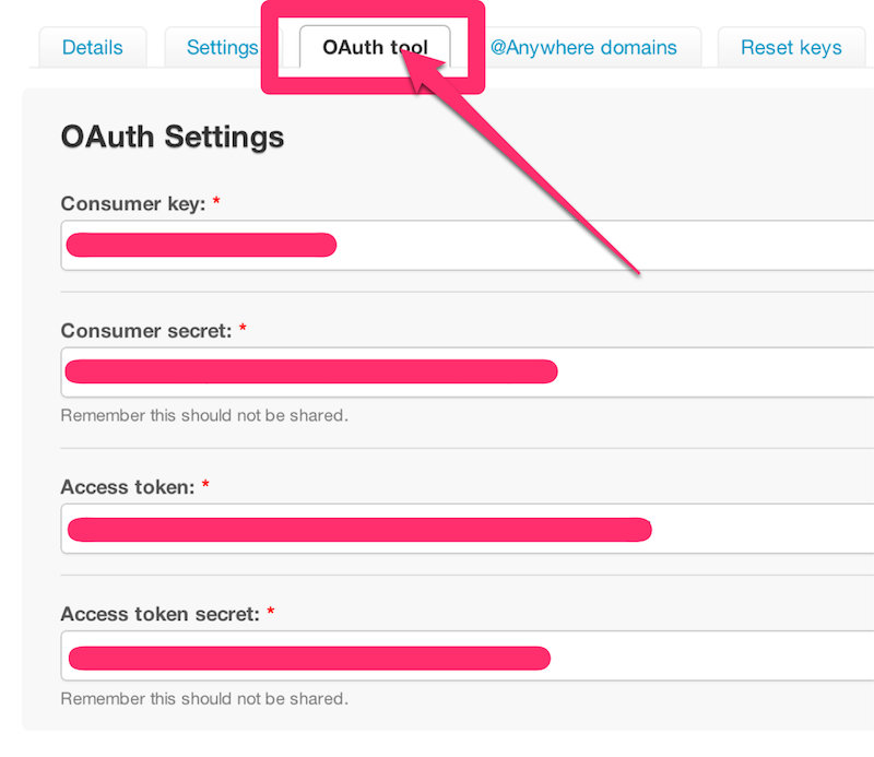
% cat config/initializers/omniauth.rb
Rails.application.config.middleware.use OmniAuth::Builder do
  provider :twitter, '[Consumer key]', '[Consumer secret]'
end

[Consumer key]と[Consumer secret]は上で取得したものを設定

スキーマ参照してモデルの設定

https://github.com/intridea/omniauth/wiki/Auth-Hash-Schema

rails g model user provider:string uid:string name:string screen_name:string
rake db:migrate

% cat app/models/user.rb 
class User < ActiveRecord::Base
  def self.create_with_omniauth(auth)
    create! do |user|
      user.provider = auth['provider']
      user.uid = auth['uid']
      user.name = auth['info']['name']
      user.screen_name = auth['info']['nickname']
    end
  end
end

セッション（ログイン・ログアウト）の設定

rails g controller sessions

% cat app/controllers/sessions_controller.rb
class SessionsController < ApplicationController
  def callback
    auth = request.env["omniauth.auth"]
    user = User.find_by_provider_and_uid(auth["provider"], auth["uid"]) || User.create_with_omniauth(auth)
    session[:user_id] = user.id
    redirect_to root_path, :notice => "Logged in"
  end

  def destroy
    session[:user_id] = nil
    redirect_to root_path, :notice => "Logged out"
  end
end

Welcomeページの設定

rails g controller welcome index

% cat app/views/layouts/application.html.erb
<!DOCTYPE html>
<html>
    <head>
        <title>Omniauth</title>
        <%= stylesheet_link_tag    "application", :media => "all" %>
        <%= javascript_include_tag "application" %>
        <%= csrf_meta_tags %>
    </head>
    <body>
        <% if current_user %>
            <%= current_user.name %>
            <%= current_user.screen_name %>
            <%= link_to 'Log out', logout_path %>
        <% else %>
            <%= link_to 'Log in', '/auth/twitter' %>
        <% end %>
        <%= yield %>

    </body>
</html>

アプリケーションコントローラ

% cat app/controllers/application_controller.rb
class ApplicationController < ActionController::Base
  protect_from_forgery

  def login_required
    if session[:user_id]
      @current_user = User.find(session[:user_id])
    else
      redirect_to root_path
    end
  end

  helper_method :current_user

  private
  def current_user
    @current_user ||= User.find(session[:user_id]) if session[:user_id]
  end
end

ルーティングの設定

% cat config/routes.rb
Omniauth::Application.routes.draw do
  get "welcome/index"
  match "/auth/:provider/callback" => "sessions#callback"
  match "/logout" => "sessions#destroy", :as => :logout
  root :to => 'welcome#index'
end

参考

April 19, 2012

MacのWeb共有でPythonのCGIを実行する環境

ユーザhogeが~/Sites以下での実行環境 .pyで実行する場合
Uncheck System Preferences > Sharing > Web Shearing
% diff /etc/apache2/httpd.conf /etc/apache2/httpd.conf.default
145c145
< LoadModule python_module libexec/apache2/mod_python.so
---
> #LoadModule python_module libexec/apache2/mod_python.so
469c469
< AddHandler cgi-script .cgi .py
---
> #AddHandler cgi-script .cgi
% diff /etc/apache2/users/hoge.conf /etc/apache2/users/hoge.conf.default
2c2
< Options Indexes MultiViews ExecCGI
---
> Options Indexes MultiViews
Check System Preferences > Sharing > Web Shearing
/Users/hoge/Sites% cat hello.py
#!/usr/bin/python
# -*- coding: utf-8 -*-

print "Content-Type: text/plain"
print
print "Hello world!"
/Users/hoge/Sites% chmod 755 hello.py
http://localhost/~hoge/hello.py にアクセスするとHello world!と表示される

April 5, 2012

LionでFinderのフォルダや選択したテキストからターミナルを開く

LionでFinderのフォルダや選択したテキストからターミナルを開くには，cdtoを利用する方法もありますが，元から入っている機能を利用して実現できます．以下はosx - Open terminal here in Mac OS finder - Stack Overflowの適当な訳．

Mac OS X Lion 10.7ではサービスを利用してターミナルを開く方法がある．デフォルトだと無効になっているので有効にする必要がある．

System Preferences → Keyboard → Keyboard Shortcuts → Services

でNew Terminal at Folder，New Terminal Tab at Folderを有効にする．日本語だとなんと表記されているかわかりません←

サービスのサブメニュー（メニューバーにあるアプリケーション名をクリックすると表示される）とコンテキストメニュー（フォルダか選択されたパス上で右クリックする）に表示される．ショートカットキーも割り当てられる．

これらのサービスは他のアプリケーションでも利用可能．またこれらはどこかのフォルダだけでなく，選択されたテキストの絶対パスからもターミナルを開ける．

フォルダを選択して右クリックでもいける

テキストを選択した状態でメニューバーからサービスを選んでもいける

さらにLionのターミナルではフォルダかパス名をターミナルのアイコンにドラッグアンドドロップすればFinderの新しいタブで開ける．

選択したテキストをドラッグアンドドロップしてもいける

フォルダかパス名をターミナルのタブバーにドラッグすると，自動的に"cd"コマンドが実行される．（単純にターミナルにドラッグした場合はパス名が挿入される）

選択したテキストでもいける

元記事にはシェルスクリプトでこれらを実現する方法や，関連情報としてサービスで選択したテキストのmanを見る方法も記されています．

March 13, 2012

KDD Cup 2012, Track 1の訳

追記

提出方法が追記されました．

追記終わり

KDD Cup 2012は3/15から．Track 1は

訓練データ（ユーザとアイテムとユーザがアイテムをフォローしたかどうか）とユーザ・アイテムのデータを使って，テストデータ（ユーザとアイテム）が与えられてたら推薦度を推定する，

というタスク．http://www.kddcup2012.org/c/kddcup2012-track1 をざっくり翻訳．誤訳なければいいけど．Tencent WeiboはTwitterとだいぶ似てるけどちょっと違うみたい．

データセット

Item, Tweet, Retweet, Comment, Followee/Followerの定義とデータセットについて．

Item

アイテムはTencent Weiboのユーザ．ユーザは個人とか組織とかグループ．アイテムはカテゴリに整理されている．カテゴリは階層構造をもつ．

たとえば Dr. Kaifu LEE, http://t.qq.com/kaifulee は

X.science-and-technology.internet.mobile
X.business.Invest.Angel Investment

の２つのカテゴリに属している．Xはルートカテゴリ．

階層は「.」で区切られていて，カテゴリの情報はモデル推定に使えるかも．たとえばPeterさんがkaifuleeさんをフォローしてる時，Peterさんはkaifuleeさんが属しているカテゴリのアイテムに興味ありそう，ついでにkaifuleeさんのカテゴリの親カテゴリのアイテムにも興味ありそうだとか．

マイクロブログのメッセージのアクション．投稿されたメッセージそのもの．

Retweet

ユーザは他のユーザのツイートにコメントをつけてリツイートできる．フォローされてるほかのユーザに共有．

Comment

ツイートに対してコメントできる．コメントは他のユーザにはプッシュされない．コメント履歴には残る．Twitterにはないかな？

Followee/follower

AがBをフォローしてたら，AはBのフォロワー(follower)，BはAのフォロウィー(followee)．

データセットについて

データセットはユーザに対するアイテムの推薦とフォローの履歴．めちゃでかい．プロフィールやソーシャルグラフ，アイテムカテゴリの情報といった様々なドメインの情報がある．

データセット内のユーザの数は数百万．いろんな情報（デモグラフィック，プロフィールキーワード，フォローヒストリーとか）があるから，いい推定モデルできるんじゃないかな．ユーザのプライバシーを守るため，ユーザとアイテムのIDは匿名化してる．更に，情報は，中国語の場合でも，ランダムな番号にしてる．だから中国語わかんなくてもカンケーない．推薦のタイムスタンプは与えられてます．

ファイル

７つのテキストからなる２つのデータセット．各項目はタブ区切り．

a) 訓練データ　rec_log_train.txt
b) テストデータ　rec_log_test.txt

(UserId)\t(ItemId)\t(Result)\t(Unix-timestamp)

(UserId) : ユーザID
(ItemId) : アイテムID
(Result) : 1か-1．1はUserIdが推薦されたアイテムItemIdをアクセプトしてフォローしたもの．-1はリジェクト．テストデータのResultは全部-1に設定されている．
(Unix-tmiestamp) : タイムスタンプ

% head rec_log_train.txt 
2088948 1760350 -1 1318348785
2088948 1774722 -1 1318348785
2088948 786313 -1 1318348785
601635 1775029 -1 1318348785
601635 1902321 -1 1318348785
601635 462104 -1 1318348785
1529353 1774509 -1 1318348786
1529353 1774717 -1 1318348786
1529353 1775024 -1 1318348786
1853982 1760403 -1 1318348789

c) ユーザとアイテムのデータ

i. ユーザプロフィール user_profile.txt

(UserId)\t(Year-of-birth)\t(Gender)\t(Number-of-tweet)\t(Tag-Ids)

(UserId) : ユーザID
(Year-of-birth) : 生まれ年．サービスに登録した時に選択
(Gender) “0, 1, 2” : わからない，男，女
(Number-of-tweet) : ツイートの数
(Tag-Ids) : 興味のあること．ユーザが選ぶ．山登りに興味があったら「山登り」を選ぶ．何も選ばない人もいる．「tag-id1;tag-id2;...;tag-idN」ってフォーマット．なにも選ばなかったら「0」

% head user_profile.txt 
100044 1899 1 5 831;55;198;8;450;7;39;5;111
100054 1987 2 6 0
100065 1989 1 57 0
100080 1986 1 31 113;41;44;48;91;96;42;79;92;35
100086 1986 1 129 0
100097 1981 1 75 0
100100 1984 1 47 71;51
100101 2003 1 31 0
100116 1988 2 39 35
100117 2009 2 37 0

ii. アイテム item.txt

(ItemId)\t(Item-Category)\t(Item-Keyword)

(ItemId) : アイテムID
(Item-Category) “a.b.c.d” : 階層的なカテゴリ．aはbの親カテゴリ…
(Item-Keyword) “id1;id2;…;idN” : キーワード．ウェイボの対応したプロフィールから抽出．数字．

% head item.txt 
2335869 8.1.4.2 412042;974;85658;174033;974;9525;72246;39928;8895;30066;2245;1670;85658;174033;6977;6183;974;85658;174033;974;9525;72246;39928;8895;30066;2245;1670;85658;174033;6977;6183;974
1774844 1.8.3.6 31449;517124;45008;2796;79868;45008;202761;2796;101376;144894;31449;327552;133996;17409;2796;4986;2887;31449;6183;2796;79868;45008;13157;16541;2796;17027;2796;2896;4109;501517;2487;2184;9089;17979;9268;2796;79868;45008;202761;2796;101376;144894;31449;327552;133996;17409;2796;4986;2887;31449;6183;2796;79868;45008;13157;16541;2796;17027;2796;2896;4109;501517;2487;2184;9089;17979;9268
1775000 1.4.2.4 259580;626835;12152;6183;561;10666;12152;6183;561;60774;21206;561;160212;539;2225;320443;12152;6183;561;10666;12152;6183;561;60774;21206;561;160212;539;2225;320443
1775024 1.4.1.4 498354;61029;60774;12318;3825;465;5788;6183;561;61029;539;71940;335;27;60774;12318;3825;465;5788;6183;561;61029;539;71940;335;27
1774455 1.4.1.2 155009;345081;12203;6183;561;9642;12203;561;3203;40075;539;345081;26124;10638;490970;12203;6183;561;9642;12203;561;3203;40075;539;345081;26124;10638;490970
1775040 1.4.2.2 100947;97714;12203;6183;3203;45782;12203;3203;46868;13;97714;12203;6183;3203;45782;12203;3203;46868;13;97714
1774505 1.4.9.2 254337;195099;974;12203;6183;974;11354;12203;974;37888;17713;62372;454;974;12203;6183;974;11354;12203;974;37888;17713;62372;454;974
1774776 8.1.4.2 239661;974;46479;17713;974;14461;46479;17713;974;31325;610;46441;143118;208450;5647;35944;70488;307170;175621;326588;46479;17713;974;14461;46479;17713;974;31325;610;46441;143118;208450;5647;35944;70488;307170;175621;326588
495072 8.1.4.2 296259;596521;4861;4385;31325;31693;12152;974;35133;205881;474444;1100;115394;76462;636390;112571;75629;4861;35639;4385;31325;136353;87610;93388;159442;146683;300971;4861;4385;31325;31693;12152;974;35133;205881;474444;1100;115394;76462;636390;112571;75629;4861;35639;4385;31325;136353;87610;93388;159442;146683;300971
2076876 1.4.9.2 239661;974;428257;6183;68271;974;6254;46479;17713;36169;6183;68271;974;50048;68271;125744;41791;30825;31325;46479;17713;60765;490251;3824;22793;102745;288673;6183;68271;974;6254;46479;17713;36169;6183;68271;974;50048;68271;125744;41791;30825;31325;46479;17713;60765;490251;3824;22793;102745;288673

iii. アクション user_action.txt

(UserId)\t(Action-Destination-UserId)\t(Number-of-at-action)\t(Number-of-retweet )\t(Number-of-comment)

(UserId) : ユーザID
(Action-Destination-UserId) : 相手のユーザID
(Number-of-at-action) : アクションの数
(Number-of-retweet ) : リツイートの数
(Number-of-comment) : コメントの数

たとえば

“A B 3 5 6”

だったら，AのBへの @つきアクション（リプライ？メンション？）が3回，リツイート5回，コメントが6回．

% head user_action.txt 
1000004 1000004 0 3 4
1000004 1290320 0 3 0
1000004 1675399 0 1 0
1000004 1760423 0 1 0
1000004 1774718 0 1 0
1000004 1774862 0 1 0
1000004 1775076 0 1 0
1000004 1837210 0 1 0
1000004 1928681 0 1 0
1000004 1954203 0 1 0

iv. ユーザSNS user_sns.txt

ユザーのフォロー履歴

(Follower-userid)\t(Followee-userid)

(Follower-userid) : フォローしたユーザのID
(Followee-userid) : フォローされたユーザのID．

% head user_sns.txt 
1000001 373407
1000001 461001
1000001 692475
1000002 1760423
1000002 1760426
1000002 1760642
1000002 1774712
1000002 1774861
1000002 1774957
1000002 1774963

v. ユーザキーワード user_key_word.txt

ツイート，リツイート，コメントから抽出したキーワード

(UserId)\t(Keywords)

(UserId)
(Keywords) “kw1:weight1;kw2:weight2;…kw3:weight3” : weightが大きいほどユーザは興味が有りそう．Integer．

% head user_key_word.txt 
1000000 183:0.6673;2:0.3535;359:0.304;363:0.1835;377:0.1831;10:0.1747;58:0.1725;127:0.1624;459:0.1482;54:0.142;330:0.1361;1480:0.1358;40:0.1136;672:0.1037
1000001 92:1.0
1000002 112:1.0
1000003 154435:0.746;30:0.3902;220:0.2803;238:0.2781;232:0.2717;1928:0.2479
1000004 118:1.0
1000005 157:0.484;25:0.4383;198:0.3033;185:0.3012;31:0.2991;80:0.2971;203:0.241;34:0.2347;95:0.2327;37:0.214
1000006 277:0.7815;1980:0.4825;146:0.175;103:0.1475;83:0.1382;107:0.1061;892:0.1019
1000007 4069:0.6678;2557:0.6104;137:0.4261
1000008 16:0.7164;154:0.3278;164:0.3222;246:0.2258;17:0.1943;14:0.1789;340:0.1789;366:0.1719;139:0.1587;279301:0.1139;484:0.1083;116:0.1055;193:0.1027

出力

各テストデータに対して

(UserId)\t(ItemId)\t(Prediction)

(UserId) : ユーザID
(ItemId) : アイテムID
(Prediction) : -1 ~ 1の値．点数が高いほど，より推薦されやすい．

評価

平均適合率で量る

ap@n = Σ k=1,...,n P(k) / (number of items clicked in m items)

分母が0だったら結果は0
P(k)はkで足切りしたアイテムの適合率．つまりk番目までのアイテムの中でクリックされたアイテムの割合．一つもフォローされてなかったらP(k)は0
n=3がデフォルト

たとえば

5つのアイテムが推薦されて，ユーザが1,3,4番目をクリックしたら， ap@3 = (1/1 + 2/3)/3 ≈ 0.56
4つのアイテムが推薦されて，ユーザが1,2,4番目をクリックしたら ap@3 = (1/1 + 2/2)/3 ≈ 0.67
3つアイテムが推薦されて，ユーザが1,3番目をクリックしたら ap@3 = (1/1 + 2/3)/2 ≈ 0.83

各ユーザに対する平均適合率平均がスコア

AP@n = Σ i=1,...,N ap@ni / N

いまいちどうやって出力したらいいかわからん．テストデータは3/15公開．

提出方法

The rec_log_test.txt にはリーダーボード（順位表）用セットと評価用セットが含まれている．ファイルは一時的にソートされている．タイムスタンプが1321891200未満のデータはリーダーボードに用いられ，1321891200以上のデータは評価に用いられる．ゴールはそれぞれのセットの中であるユーザに推薦されたアイテムがユーザによってフォローされかどうかを推定してやること．

出力サンプルはダウンロード可．2種類のフォーマットが利用できる．一つはヘッダあり2列のcsvファイル（サイズは大きくなる）．一つはヘッダなし1列のcsvファイル（サイズは小さくなる）．圧縮して提出することが望ましい．アップロードされたら10〜20秒後にリーダーボード用のデータにスコアが付けられ，結果がリーダーボードに表示される．

2列csvフォーマットでは，1列目はユーザID（リーダーボード用，評価用，それぞれでソートされている），2列目は0~3個のスペース区切りの推薦すべきアイテムID(e.g. "647356 458026 1606609")を．n=3の平均適合率が計算される．提出ファイルのユーザIDの順番はサンプルと同じ順番に正確に対応させなくてはならない．すなわち，リーダーボードセットの結果は評価セットの前におき，それぞれのデータ内ではユーザIDでソートされていなくてはならない．

1列フォーマットでは，単純にスペース区切りでアイテムを．順番は2列の場合と同じ．

% head rec_log_test.txt
1449438 1394821 0 1321027200
1449438 372323 0 1321027200
1525431 1774707 0 1321027200
1587150 1774422 0 1321027200
1587150 1774934 0 1321027200
2064344 1505267 0 1321027200
2081969 1760410 0 1321027200
2141596 1760376 0 1321027200
2359607 1606609 0 1321027200
2359607 2105484 0 1321027200

2列

% head sub_small_header.csv 
id,clicks
100001,647356 458026 1606609
100004,647356 1606574 1774568
100005,1606574 1774532 586592
100009,647356 1760327 1606574
100010,458026 2105511 713225
100011,1774594 1774717 1774505
100012,458026 2105511 727272
100013,1870054 514413 1760401
100014,859545 2167615 715470

1列

% head sub_min.csv 
647356 458026 1606609
647356 1606574 1774568
1606574 1774532 586592
647356 1760327 1606574
458026 2105511 713225
1774594 1774717 1774505
458026 2105511 727272
1870054 514413 1760401
859545 2167615 715470
647356 458026 1606574

February 17, 2012

Pythonで線形動的システムのパラメータ推定を実装してみるもなんかうまくいってない

線形動的システム（線形力学系，Linear dynamical systems; LDS）のEMアルゴリズムによるパラメータ推定を行いました．が，うまくいってない気がします．カルマンフィルタなどで扱う状態方程式（外部入力なし）と観測方程式において，状態と観測が与えられたときに，係数を求めるのが目的です．Ghahramaniらの論文 ¹の手法を実装します．

状態方程式と観測方程式が

$\begin{align}
{\bf x}_{t+1}&=A{\bf x}_t + {\bf w}_t\\
{\bf y}_{t}&=C{\bf x}_t + {\bf v}_t\\
{\bf w}_t &\sim N(0,Q)\\
{\bf v}_t &\sim N(0,R)\\
\end{align}$

というように表され，$\{{\bf y}_1,...,{\bf y}_T\}$が与えられたときに，$A,C,Q,R$と初期状態の平均ベクトル$\pi_1$と分散共分散行列$V_1$を推定します．

論文がとても分かりやすいので，実装に必要なところだけ抜粋します．

Eステップ

以下のように定義します．

$\begin{align}
{\bf x}_t^{\tau}&=E({\bf x}_t|\{{\bf y}_1^{\tau}\})\\
V_t^{\tau}&=Var({\bf x}_t|\{{\bf y}_1^{\tau}\})\\
\end{align}$

Kalman filter

$\begin{align}
{\bf x}_1^0 &= {\bf \pi}_1\\
V_1^0 &= V_1\\
{\bf x}_t^{t-1} &= A {\bf x}_{t-1}^{t-1}\\
V_t^{t-1} &= A V_{t-1}^{t-1} A' + Q\\
K_t &= V_t^{t-1}C'(CV_t^{t-1}C'+R)^{-1}\\
{\bf x}_t^t &= {\bf x}_t^{t-1} + K_t({\bf y}_t-C{\bf x}_t^{t-1})\\
V_t^t &= V_t^{t-1} - K_t C V_t^{t-1}\\
\end{align}$

Kalman smoother

$\begin{align}
J_{t-1} &= V_{t-1}^{t-1}A'(V_t^{t-1})^{-1}\\
{\bf x}_{t-1}^T &= {\bf x}_{t-1}^{t-1} + J_{t-1}({\bf x}_t^T - A{\bf x}_{t-1}^{t-1})\\
V_{t-1}^T &= V_{t-1}^{t-1} + J_{t-1}(V_t^T - V_t^{t-1})J_{t-1}'\\
V_{T,T-1}^T &= (I - K_T C)AV_{T-1}^{T-1}\\
V_{t-1,t-2}^T &= V_{t-1}^{t-1}J_{t-2}' + J_t-1(V_{t,t-1}^T - AV_{t-1}^{t-1})J_{t-2}'\\
\end{align}$

これらを用いて，Mステップへの入力を求めます．

$\begin{align}
{\hat {\bf x}}_t & = {\bf x}_t^T \\
P_t & = V_t^T + {\bf x}_t^T {{\bf x}_t^T}' \\
P_{t,t-1} & = V_{t,t-1}^T + {\bf x}_t^T{{\bf x}_{t-1}^T}' \\
\end{align}$

Mステップ

$\begin{align}
C^{new} & = (\sum_{t=1}^T {\bf y}_t {\hat{\bf x}}_t')(\sum_{t=1}^T P_t)^{-1} \\
R^{new} & = \frac{1}{T}\sum_{t=1}^T({\bf y}_t{\bf y}_t' - C^{new}{\hat{\bf x}}_t{\bf y}_t') \\
A^{new} & = (\sum_{t=2}^T P_{t,t-1})(\sum_{t=2}^T P_{t-1})^{-1} \\
Q^{new} & = \frac{1}{T-1}(\sum_{t=2}^T P_{t} - A^{new}\sum_{t=2}^T P_{t-1,t}) \\
{\bf \pi}_1^{new} & = {\hat {\bf x}}_1 \\
V_1^{new} & = P_1 - {\hat {\bf x}}_1{\hat {\bf x}}_1'
\end{align}$

なおN個の観測列があるときは

$\begin{align}
{\bar {\hat {\bf x}}}_t & = \frac{1}{N}\sum_{i=1}^N {\hat {\bf x}}_t^{(i)} \\
V_1^{new} & = P_1 - {\bar {\hat {\bf x}}}_1{\bar {\hat {\bf x}}}_1' + \frac{1}{N}\sum_{i=1}^N [{\bar {\hat {\bf x}}}_1^{(i)}-{\bar {\hat {\bf x}}}_1][{\bar {\hat {\bf x}}}_1^{(i)}-{\bar {\hat {\bf x}}}_1]' \\
\end{align}$

実験

Wikipediaのカルマンフィルタの例にあるシステムで実験してみました．トロッコが摩擦なしの無限レール上でランダムな力によって動くシステムです．

データを生成するために用意したパラメータは

A
[[ 1.   0.1]
 [ 0.   1. ]]
C
[[ 1.  0.]]
Q
[[  2.50000000e-05   5.00000000e-04]
 [  5.00000000e-04   1.00000000e-02]]
R
[[ 1.]]

でした．

が，下のコードによって推定された結果は

A
[[ 0.62656567  0.64773696]
 [ 0.56148647  0.0486408 ]]
C
[[ 0.19605285  1.14560846]]
Q
[[ 0.15479875 -0.12660499]
 [-0.12665761  0.31297647]]
R
[[ 0.59216228]]
pi_1
[[-0.39133729]
 [-0.89786661]]
V_1
[[ 0.18260503 -0.07688508]
 [-0.07691364  0.20206351]]

でした．下のコードでは生成されるデータは毎回異なるので結果はその都度変わります．がどうもうまくいかない．

赤が真の位置，マゼンダが推定された位置．青が真の速度，シアンが推定された速度．

どこがおかしいのだろう(:D)|￣|_ =3

1. Z. Ghahramani and G.E. Hinton. Parameter estimation for linear dynamical systems. University of Toronto technical report CRG-TR-96-2, 6, 1996.

February 1, 2012

Xcode 4でPythonの開発環境を整える

XcodeでPythonを開発することができるようです．はじめは少々面倒かもしれませんが．でもXcodeのPythonシンタックスハイライトはきれいな気もするし，Emacs風のキーバインドも使えるし，アリかも．

Python in Xcode 4 - Stack Overflowを~~訳しただけ~~参考にしました．

Xcode 4を開く．
"File" → "New" → "New Project…"で新しいプロジェクトを作成．
"Mac OS X"の"Other"を選択．
"External Build System"を選択し，"Next"をクリック．
プロダクト名と識別名（Company Identifier）を入力．
"Build Tool"には，/usr/bin/pythonを入力して"Next"をクリック．ほかの場所にPythonをインストールしてたらそれを入力．
どこに保存するか決めて"Create"．
メニューバーから"File" → "New" → "New File…"を選択．
"Mac OS X"の"Other"を選択．
"Empty"を選択し，"Next"をクリック．
拡張子".py"を含んだPythonファイルをプロジェクトのフォルダに保存し"Save"をクリック．
メニューバーから"Product" → "Edit Scheme…"を選択．
左のコラムから"Run"を選択．
"Info"タブから，"Executable"フィールドを選択し，"Other…"を選択．
手順6で選んだ場所に移動．⇧⌘G （shift + command + g）で移動する場所を指定できる．
"Executable"から選択．
"Debugger"フィールドは，"None"を指定．
"Arguments"タブから"Base Expansions On"フィールドを選択，プロジェクトの名前を選択．
"Arguments Passed On Launch"の"+"をクリック．
$(SOURCE_ROOT)/実行したいファイル名を記入．ファイルはプロジェクトフォルダの中にないと実行できない．もしほかの場所のものを実行したいときはフルパスを記入．スペースを含む場合はクォーテーションで囲む．
"OK"をクリック．
コーディングをはじめましょう！

⌘Rで実行できます．
デフォルトでは出力は下のパネルに表示されます．
タブ幅，文字コードは右のパネルから変更可能です．
Pythonの自動インデントはできません．
応用すれば他の言語の開発環境もつくれるかも．

Macbook Airの環境を整える覚書その２

自分用．以前書いたMacBook Airの環境を整える覚書と合わせて．

Finder

サイドバーの文字サイズ変更

System Preferences > GeneralでSidebar icon sizeをSmallに．
ついでにRestore windows when quitting and re-opening appsはアンチェック．

Terminal

ログインシェルをzshに変更

System PreferencesからUsers & Groups
左下のロックを外して，Current Userを右クリック，Advanced Options...
Login shellを/bin/zshに．

行数の変更，終了後の動作の変更，metaキーの設定の変更

PreferencesからWindowでRowsを43に．

PreferencesからShellでWhen the shell exits:をClose if the shell exited cleanlyに．

PreferencesからKeyboardでUse option as meta keyにチェック．

キーボード

フルキーボードアクセスをすべてのコンポーネントで．ダイアログでタブとスペースを組み合わせて選択できるようになる．

IME

Input Sources

System Preferences > Language & Text > Input SourcesからDvorak - Qwerty ⌘，Kotoeri > Hiragana，Romajiの3つを選択．ときどき気が向いたらDvorak←
ついでにKeyboard & Character Viewerにもチェック．
2つ以上のInput Sourceの切り替えは⌘長押しで．

Google 日本語入力

すばらしいんだけどDvorakとうまく共存できない…？

App Store

Xcode

開発環境．ダウンロード後，Install Xcodeを実行．

Stuffit Expander

解凍．

The Unarchiver

解凍．

Evernote

メモ．

Skitch

スクリーンキャプチャ．

パッケージ管理

Homebrew

MacPortsより楽な気がする．

/usr/bin/ruby -e "$(curl -fsSL https://raw.github.com/gist/323731)"

要Intel CPU，OS X 10.5 or higher，Xcode with X11，Java Developer Update．

フォント

Ricty

Incosolata + Migu 1M．Terminalに開発環境に．RictyをインストールするためにはFontForgeを入れる必要があります．

brew install fontforge
ln -s /usr/local/Cellar/fontforge/20110222/FontForge.app /Applications

2行目のシンボリックリンクの張り方はFontForgeインストール後に表示される．

テキストエディタ

CotEditor

Preferences > Syntax > Delay coloringにチェック

ウェブブラウザ

Chrome

AdBlock Plus
広告除去．日本向けフィルタを購読．
LastPass
パスワード管理
Mail Checker Minus
Gmailチェック
Better History
履歴を使いやすく
Google Reader Open entry in background tab
Google Readerの記事をバックグラウンドで開く
Language Links for Google
Googleをワンクリックで言語切り替え
Deny Rakuten News
楽天メルマガ解除

Firefox

Opera

LaTeX

UpTeX.app

色々まとまって入ってる．

ghostscript

Homebrewインストール後

brew install ghostscript

TexShop

LaTeX書くときは便利．テキストエディタで書いちゃうことも多い．

ファイル共有

Dropbox

よほど大きくならない限り計算結果なんかもここに．持ってるすべての端末でzsh, vim, emacs, CotEditorの環境設定も共有．~/Dropbox/Settings以下に共有する環境設定を置いておく．下は環境共有をまとめて設定するシェルスクリプト．つったってシンボリックリンク貼ってるだけ．

Python

pip

Python用パッケージ管理．http://www.pip-installer.org/en/latest/index.html

easy_install pip

easy_installのかわり．アンインストールもできる．

ScipySuperpack

Lionの環境に合わせたscipyやら入れるために．